Multi-Armed Bandits: The Scientific Shotgun for Evals
Introduction: Escaping the AI Agent Evaluation Hamster Wheel
Speaker G opens by describing the endless cycle of maintaining and improving AI agent quality—tracking model updates, user requests, drifting evals, and degrading tool calling. He promises a way to get faster results, reduce bad outputs served to users, and save money, setting up the talk's focus on data science techniques applied to AI agents.
AB Testing Basics and Its Limitations
The speaker gives a quick refresher on AB testing—serving different product variations to different users for a fixed duration—and highlights its key flaw: being locked into a split even after early evidence shows one variation is clearly worse, leading to wasted user experience during the experiment's remaining duration.
Introducing Multi-Armed Bandits
Speaker G introduces multi-armed bandits as the talk's central concept, explaining the origin of the term from slot machines ('one-armed bandits') and how the algorithm family navigates uncertainty by dynamically choosing among multiple variations, unlike static AB testing.
Epsilon Greedy Algorithm Explained
Using a customer support chatbot tone-of-voice example (formal, warm, direct, playful), the speaker explains the epsilon-greedy algorithm, where the best-performing variation is chosen most of the time (exploitation) while occasionally sampling other variations at random (exploration) to avoid premature commitment.
Visualizing Epsilon Greedy vs Traditional AB Testing
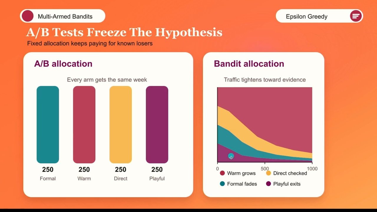
Speaker G walks through side-by-side graphs comparing traditional AB testing to epsilon-greedy over a week-long experiment, showing how epsilon-greedy dynamically shifts traffic toward the popular 'warm' tone and away from the unpopular 'playful' tone, resulting in better outcomes for users regardless of when the experiment is stopped.
Thompson Sampling: A More Advanced Bandit Algorithm
The speaker introduces Thompson sampling as a more sophisticated bandit algorithm that uses posterior probability distributions built from observed data to adjust exploration dynamically, rather than maintaining a fixed exploration rate like epsilon-greedy. Graphs illustrate how confidence in the best variation (the 'warm' tone) sharpens as more conversations are observed, from 50 to 1,000 samples.
The Jelly Bean Analogy for Statistical Confidence
Speaker G uses a jelly bean jar analogy to illustrate p-values and statistical confidence, showing how quickly one can become confident about a result (e.g., five fruit-flavored jelly beans in a row) without exhausting a fixed sample size, reinforcing why algorithms like Thompson sampling improve on rigid AB testing and epsilon-greedy approaches.
Applying Bandit Algorithms to Offline Evals
The speaker extends the multi-armed bandit framework to offline evals, explaining how running LLM-as-judge evaluations across thousands of prompts and multiple models can be costly, and proposes setting a confidence budget instead of a fixed prompt count to stop testing once statistical confidence in the best model/configuration is reached.
Validating Confidence with Bayesian Methods and Cohen's Kappa
Speaker G discusses using Bayesian theory to set initial values for bandit-based evals and introduces Cohen's kappa as a way to validate whether the bandit-derived results align with traditional evaluation methods, ensuring the approach's validity before scaling it up.
Closing Thoughts: Old Science, New Applications
The speaker wraps up by emphasizing that multi-armed bandit theory is well-established, proven data science—not a new invention—but is newly relevant for optimizing AI agent harness variations and offline eval suites. He closes by reaffirming the value of applying classical statistical methods within modern AI and neural network systems, then shares contact information.
Alright. If any of you are involved at all in maintaining or improving the quality of AI agents, you're likely aware that being on the data flywheel can feel like a never ending hamster wheel. You got new model versions landing. Your users are asking for new tasks. Your evals are drifting. Your tool calling degrades. But you do care, so you keep working at this.
You're reading your traces. You're iterating on your system prompts. You're finagling your harness. What if I told you that all of those things are still things you have to take care of, but you can get results faster. You can serve users fewer bad outputs, and you could even save some money. Sound good to you guys?
Alright. Every time I talk about data science, there's this tension I have between how much of algorithms on the blackboard I show and how quickly we can get to the fun blowing stuff up of the science part. So I know that this room is a jar of the smartest cookies in the industry. So I'll assume you guys can look stuff up in your own time. And I won't bore you with too much of the underlying math. But instead, I'll show up all the exact terminology so that you can take a photo of it, write it down, make a mental note, whatever. So with housekeeping over, let's start off with AB testing.
Now ad testing, that's not where you do sit ups and crunches and count how many you can do. A lot of you have used it before but I'll do a very very quick overview. It's where you serve different variations of parts of your product to different users. That's all it is. It could be a different call to action button.
It could be different wording in your copy. And for us, different pieces of your agent harness. The thing about AB testing is that usually it's for a fixed duration. You say you set it for a week, whether your users prefer version a more or version b or potentially even c d e and so on. One thing about AB testing is that you're locked in once you make that split. Say you have this cool loading spinner and you're showing that to half of your users.
What if on day one of your one week experiment you can already tell that that it's painfully obvious everyone hates variation a. All I want is a slice of that sexy new variation b. For six days, you're just like breeding that hatred in your users and serving half of them something that you already know yourself they don't want. What do we do about that?
Well, the main character of this talk, multi armed bandits. Why are they called that? Well, another name for the pokey machines or a slot machine is a one armed bandit because that, lever there is an arm and it takes your money. Don't gamble. Multi arm bandits on the other hand related to this because we have multiple levers we can pull for different variations kind of like a b c d e f g taste testing.
And the reason why they chose poky machines as this analogy is because multi armed bandits are all about navigating uncertainty. And if there's anything about gambling, it's that it's uncertain other than the fact that you're certain to lose money. In order I did say I'm not gonna go too hard into the math, so I'll just lightly give you an example of how we're gonna walk through this.
I'm gonna show you how a typical AB experiment will work over a week and how it would work with a very basic multi armed bandit algorithm. So in this scenario, you've got a customer support chatbot that's fed through one of your agents, and we're trying to test different tones of voice and see which one's better, whether it's, like, very formal, like a bit of warm, more direct language, or something really playful. And you can see there in ABCD, I've written some percentages there. For our educational purposes, we have a crystal ball and we know genuinely what users actually like more or less.
The winner clearly is warm at 70% and the worst is playful. With an AB test, what you would traditionally do is, okay, we have four of these arms or variations. We're gonna split 25% of our users into each of these variations. Epsilon greedy. Now that's the first bit of data science jargon I'm throwing at you guys.
That is an implementation of multi arm bandits, and it's exactly as it says there. As you have more and more samples from your users, you're gonna start seeing a picture of which one is doing better or not. So pick that one nine out of 10 times, but on that tenth time, pick another random one, and we call this exploration. So when you choose your optimal current result, that's exploitation, so you can serve your users more of your users, the good ones, but you still, you know, don't like put all your chickens all your eggs in one basket.
You still reserve about 10% of your randomization for other variations to see if it might just be you got lucky and the first 100 users, you know, first 100 conversations preferred one over the other. And that's why there's a balance and, it's a bit more flexible than traditional AP testing.
That's why it's called epsilon. It's just a random, you know, Greek number. One in 10 is what the epsilon is. So if your epsilon is point 10% is the random exploration. If your epsilon is point five, then for every second one, you choose a random one instead. Side by side, you can see a very clearly painted picture of what the difference is.
So from day one to day seven in your AB testing, you're spitting up evenly and whether, you know, we found out that warm was successful on day one or not, we're stuck with it. But if you can smudge in, all the way here left on day one or, you know, the first of your 1,000 hypothetical conversations, we do have this even split at the start because we don't know yet which one of these is optimal and which one users tend to like. But as that 70% value starts to rear its head and the 30% for playful rears its head as well, we narrow that down so playful is that dark purple one and you can see that over time because it's unpopular we start serving that to users less and less.
We see that the direct, sorry, the warm, which is a light purple, I could have chosen better colors, is popular. We start serving that more and more to users. So you can see that regardless of whether you stop the experiment early after, say, day two or whether you let it run and forget to pick one, that's optimal.
Your users oops. Your users are getting more good results instead of you having to wait to be the one who chooses that right arm. But this is better. This is a basic multi armed bandit algorithm, but we can do better. One issue oh, I was gonna say, if this is, this one highlights a lot of the basic understanding.
If you take away anything from this, take a photo of this slide. Because even though it's a basic algorithm, it illustrates, everything you need to know about multi hand burners. Did you take a photo of that slide? The right one? No. I got that. Give you one more chance.
Thank you.
You're welcome. There is an even more advanced algorithm. There are many, many algorithms, but I'm gonna show you just two today. Thompson sampling, is a slightly more clever version of epsilon greedy because, say, on day one, you can tell that that warm tone of voice was very popular.
But then if that's the case, why are we kind of going back to old a b kind of methodology where we're still, like, serving and randomly exploring all these alternative ones? Ones. On day seven, why are we still serving things to why are we still serving the playful tone of voice when we already know everyone hates it?
So what Thompson sampling does is actually take into account how many times you've actually sampled or observed a result from the users. So there's another bit of jargon there, posterior probability distribution. All that means is what you've observed from the data as you go along. So you have your prior distributions and what you believe and see before you, run your experiment, and in between each observation.
But then you observe more data, you build up your beliefs, and you update your beliefs. So imagine, in the same actually, I have fancy graphs for you here. Pretty pictures. Look at this. So after about 50 of these conversations in this chatbot, you do kinda see, like, an image of, like, what's, you know, more or less popular, but, those peaks, they're kind of similar.
You know? That's kind of, like, within a within a window of error. After about 200, the picture starts emerging a bit more, and you can see that that warm tone of voice starts to stand out amongst the rest. And by the time you get to a thousand, it's pretty clear which one is the standout winner. And rather than just spending that 10% epsilon of, like, randomly exploring all these other ones to give it the benefit of doubt, we know we don't really need to give the benefit of doubt if it's that obvious. Right?
So Thompson sampling is what you probably use, like, in production. At least it's one of the first production ready kind of algorithms you would use. Epsilon Green is just really handy to, like, explain the concept of multi armed bandits. And this stuff is pretty intuitive. Right? Like, imagine you were given a task to you had two jars of jelly beans, 10,000 each, and they've got two flavors, lime flavored and foot flavored.
And it's your job to find out which jar is more likely to have foot flavored jelly beans. They look identical except for taste. That's the only way you can discern between them. You've shaken them all about so you know that they're evenly distributed. And let's say you start having a few observations. You start taking out a jelly bean jelly bean and you get 10 in a row from jar a that are foot flavored.
And from jar b, you just get, you know, random, you know, one and two is, foot flavored, one and two is lime flavored. After you've had 10 foot flavored jelly beans in your mouth, you kinda call it a day. Right? You wouldn't just keep, like, shoving down your mouth. You'd be insane. Right? But imagine if we went with the, either AB testing mode or, simple Epsilon Greedy. You would say, okay.
Well, yeah, I get it. It seems like it seems like it's jar a that has more flavor ones, but I'm just gonna keep eating them because the experiment runs full and there are 10,000 jelly beans. For those of who know about p values, if you eat three jelly beans in a row that are full flavored, that's, like, odd but not super rare.
Four is a bit unusual, but by the time you even eat five in a row, that's already a p value of less than point zero five, which means that there's a one in 20% chance that that's just a random coincidence. This shows you kind of, like in an illustration of why you might want to build on these algorithms.
So AB testing, you get your results and it kind of stays the same of what you're serving to users. Epsilon Greedy is already an improvement. Thompson sampling takes it further by being more reason about this. And if I had 81 instead of eighteen minutes, I'd tell you about upper confidence brow upper confident upper confidence bounds rather, contextual bandits, adversarial bandits, all this.
This is all stuff you can look up. It's a fascinating world that I'm trying to convince you. It's exciting and useful for AI agents. But, of course, my talk also had the word evals in it. The same type of methodology and theory applies to offline evals as well. So say you have a suite of 1,000 prompts that you run your evals against.
It could be like just 50 golden sets and then 950 other prompts just to align your product that your PMs manage or whatever. You also know that after, you know, you've run it halfway through and you can you've got monitoring on these evals feeds running as well, yours you can also see things emerging out ahead on top of the other. But most of you, if you're doing evals, you're also doing LLMs as judges and that costs money. Right?
You can do more like test like evals that are more like deterministic and like code driven, but every LLM as a judge call costs money. And if you've got a thousand prompts and you're testing four models because Anthropics released blah blah blah 5.2 GPTs got, you know, a nice 6.7, but then you wanna try it with like low reasoning and high reasoning and all that.
For each of those, you're running 1,000, observations, and each one of those costs x number of cents when you've already gotten the picture early on. So the same thing applies to, offline evals as well. Rather than setting a budget of 1,000 prompts to assess against, set a budget of confidence. So keep running those evals until you get a picture that looks like this. You know, you've got a confidence bound of like 95% sure that GPT 5.4 with medium reasoning is the right choice for your agent.
And that's the scientific shotgun part of it as well. It applies to whether you're doing Epsilon or Thompson. The shotgun is you blast it out. You don't care on day one whether, one is better or not. If you bring in you can look this up again. Bayesian theory and Bayesian analysis with Thompson sampling. You can use, like, your prize and calculate what your initial values are, but either way, you can just start with a split 252525% start with. But then by day two, you're getting a picture.
The evidence appears, and that's when you start tightening it towards what you think is obvious, you know, and makes sense intuitively as a human as well. And then you can compare this against your own eval. Cohen's kappa, another term you can look up, whether it aligns with what you would normally see if you run your own forms of testing as well, see if it's valid or not.
And if it is, then you can run with this. Run it only as many times as you need to rather than just for the sake of picking a number of, like, 1,000 and saying, yep. That's us doing due diligence because we're running that enough. So this is all very, like, proven stuff. Like, multi armed bandits isn't something I've invented or come up with or was recent. It's like age old data science.
It's just old stuff that I'm presenting to you now. And what was once old is still old, but used in new ways such as the exploration slash exploitation of agent harness variations in online deployments and the optimized use of suites in offline evals as I've been talking about. So if I was trying to sell you snake oil, I'd probably use something more sexy than, you know, like, oh, the the posterior probability optimizes the blah blah blah blah blah blah blah.
But this is real science, real, maths that does work, and we're so used to seeing evals as an LLM as a judge process because the whole reason we have evals instead of unit tests is because we have to evaluate these, natural language problems in our space. But even in that space of natural language problems, we can use old you know, we're not running neural networks for multi ambient, but it's still relevant and applicable to the way we handle data.
So that's me. Hopefully, I've convinced you that this old, you know, ragtag multi armed bandit crazy data science concept does have place in our new world of AI and black box neural networks. You can find me via that QR code or you can type in the convenient URL of..dev.
Otherwise, you can find me on random socials of one voluted. Thank you very much.
Technologies & Tools
- GPT-5.2
Concepts & Methods
- AB Testing
- Adversarial Bandits
- Bayesian Theory
- Cohen's Kappa
- Contextual Bandits
- Epsilon Greedy
- Exploration vs Exploitation
- LLM as a Judge
- Multi-Armed Bandits
- P-value
- Posterior Probability Distribution
- Prior Distribution
- Thompson Sampling
- Upper Confidence Bound