Fail fast, fix faster: Why faster AI models beat smarter ones

Rethinking Model Performance: Speed vs. Intelligence
The speaker introduces the central thesis of the talk: once a model becomes competent enough, the speed of iteration matters more than raw intelligence. He frames the question as a shift from 'how well does a model perform' to 'how quickly can it achieve results,' setting up the exploration of new fast models that made this idea testable.
Mercury Two and the Speed-Capability Trade-off
The speaker describes his first impressions of Inception Labs' Mercury two model, noting its surprising speed and competence comparable to early 2025 models. He explains how this discovery challenged the assumption that capability must always be prioritized over speed, prompting him to explore whether a fast, lower-capability model could outperform slower frontier models.
The Ralph Wiggum Loop and Auto Research Inspiration
The speaker introduces the concept of a 'Ralph Wiggum loop'—a goal-based iterative system with good feedback mechanisms—and proposes 'speedrunning' it using fast models like Mercury two. He connects this idea to Andrej Karpathy's Auto Research release, which emphasized cheap experiments, measurable feedback, and iterative improvement, reinforcing the theoretical basis for his benchmark.
Designing the Benchmark: A Quote Approval API Task
The speaker details the engineering task used for benchmarking—a quote approval API with business rules, an OpenAPI contract, and a parallel test suite. He explains how he built an agent harness modeled on the Ralph Wiggum loop, which calls the model, implements code, runs tests, and feeds results back to the model in a repeating cycle, using instant modes for fair throughput comparisons.
Benchmark Mechanics and Live Trace Demonstration
The speaker explains the benchmark parameters—15 turns maximum, 10 runs per model, and checks for stagnation or thrashing—and then shows a live trace comparing model performance. The demonstration highlights how quickly Mercury completes the task compared to other models, setting up the deeper explanation of diffusion model speed.
Why Diffusion Models Are Faster: Autoregressive vs. Diffusion Architectures
The speaker contrasts autoregressive and diffusion model architectures, explaining that diffusion models refine outputs from noise in a small number of steps rather than sequentially generating tokens. He emphasizes that diffusion doesn't make a model smarter but drastically reduces the cost and time to produce candidate solutions, which becomes powerful when combined with fast validation loops.
The Mathematics of Compounding Iteration
The speaker explains the mathematical principle behind why fast iteration wins: each iteration removes a fraction of the remaining error, so more iterations in the same time window compound advantages. He illustrates how a less capable but fast model can outperform a slower frontier model by accumulating small incremental improvements, describing this as a 'compounding performance ratchet' that depends on cheap experiments and measurable evaluation.
Headline Results: GPT-5.4, Claude Opus, and Mercury Two Compared
The speaker presents benchmark results comparing GPT-5.4 and Claude Opus, which reliably one-shot the task but take significant time, against Mercury two, which can't one-shot the goal but completes it roughly fifteen times faster via its feedback loop. He also highlights a competence threshold below which some models never complete the task regardless of turns or runs, validating the benchmark's discriminative power.
Standout Result: GPT-5.4 Mini's Efficiency
The speaker highlights GPT-5.4 Mini as a surprising standout, achieving the same quality as its larger sibling in half the time due to more efficient distillation and inference tuning. He concludes that model choice remains important, but loop speed and quality now matter just as much as raw model intelligence in determining engineering outcomes.
Validation as the New Product Core
The speaker argues that as generation becomes fast and cheap, validation and specification become the true product, not the generated code itself. He stresses that dense, cheap, and fast feedback systems are essential to prevent autonomous agents from thrashing, drawing on his own experience debugging weak validation during benchmark setup.
Test-Driven Development as a Control System for Agents
The speaker reframes test-driven development not just as a confidence tool for human developers but as a control system enabling autonomous agents to rebuild, iterate, or optimize against a spec independently. This shift changes what validation systems can be used for, enabling parallel exploration of solutions and continuous optimization of running systems.
Caveats: Diffusion Models Aren't a Universal Replacement
The speaker cautions against wholesale replacing frontier autoregressive models with diffusion models, noting that diffusion currently lags about twelve months behind the frontier in raw capability, comparable to Gemini 2.5 Pro. He emphasizes that raw intelligence still matters greatly for tasks requiring high competence, especially for autonomous operation.
When Autonomous Loops Work and When They Break Down
The speaker explains that autonomous systems thrive with dense feedback, measurable correctness, and cheap validation, but fail when feedback is sparse or evaluation is subjective. In such ambiguous cases, he recommends using the highest-quality model available alongside techniques like LLM-as-judge or human feedback to steer the process.
Closing Recommendations and Final Thoughts
AJ Fisher wraps up by urging the audience to experiment with different model architectures, benchmark entire iteration loops rather than just output quality, and invest heavily in validation harnesses. He closes with the key takeaway that once a model clears a competence threshold, the critical question shifts from 'how smart is the model' to 'how fast is your loop,' before directing attendees to his resources and contact information.
Good afternoon. Thank you, Dave. That was, that was a great explanation. So I'm really pleased to be here this afternoon to talk to all of you about how once a model becomes competent enough, the speed of your iteration loop starts to matter far more than the headline intelligence of the model itself. So for a while now, I've had this idea that instead of focusing on how well does a model perform a task, what happens when a model gets good enough that you expect it to succeed, and instead, the benefit starts to move to how quickly it can achieve the result that you're after?
Now earlier this year, we got some new models that made this idea worth testing. And today, I'm gonna take you through some of the results of that, how I built some benchmarks to do it, and discuss some of the implications of this from an engineering perspective. So when Mercury two launched from Inception Labs, it immediately caught my attention. It stood out not just because it was fast, but it also seemed for the first time competent.
Now it was not frontier level competent, but it was comparable to an model from early twenty twenty five, and it could produce useful code in seconds. After trying it out, I was absolutely stunned. If you haven't played with it, go and play with it. It was supremely fast.
So this model seemed to be a bit of a step change in terms of the way that we think about this trade off between speed on one side and capability on the other. And thus far, we've always prioritized capability. So off the back of that, I went away, did a few calculations, and I thought, if you could produce a loop that was really quick, could you brute force your way to success?
So putting that a different way, could we speedrun a Ralph Wiggum loop? So the idea is that if I've got a lower capability model but a very reasonable rate of improvement and I can iterate quickly, in theory, I'd be able to outperform a slow, cumbersome, high performance frontier model before it's even finished its first turn.
And a Ralph loop is perfectly designed for that type of goal based system design, but assuming it's got good feedback mechanisms. So I had a look at the Mercury two performance data, and I worked out that this should make this theory at least testable to kinda, like, try this out. A couple of weeks later, Andre Carpathi releases Auto Research, which was a similar pattern but coming at it from a a different perspective.
He was thinking about cheap experiments, measurable feedback, and repeated iterative improvement. So I collected all these ideas in hand, and I went about building a bit of a benchmark and an agent harness, to test this theory out. And I'll talk you through that, now. So this was the core task.
Now this is not exhaustive in terms of a model's capability, but there's other benchmarks that will do that, and we saw some of those this morning. But this is a job that should be familiar to pretty much all of you because you've probably built something like this at some point in your careers. It's a it's a real engineering task.
So it's a quote approval API. It's got an open API contract. It's got business rules around discounts and approval thresholds and all of that sort of stuff. And it's got a whole bunch of tests that run-in parallel and take a couple hundred milliseconds to run. I then started building out a little agent harness that was modeled on a Ralph Wiggum style loop.
And this agent harness does the usual things that you would expect. It makes an API call to the model. It gets the resulting implementation, that runs the server, and it runs through the validation test suite to test how well it's performed. And as much as possible, what I'm trying to do is force the models to use their instant modes so they're running at the highest possible throughput that they can achieve, so it's comparable between different types of models. And once that's complete, the agent gets back the feedback of its turn, its current implementation so it knows where it finished, and then it's rebriefed on the goal, and the loop goes again. And they take another turn and another turn and another turn, ideally, until they finish the task.
So all of this together starts creating a benchmark. So we limit the harness to run for up to 15 turns. If it passes before that, that's great. Tick. Likewise, there's some checks in there to stop it if it starts thrashing or it gets stagnant, you know, that sort of thing. And it does 10 runs for each type of model that we wanna test. So we can get a spread of results across that, and then we get our benchmark score from there.
Now I've got some traces of this, which I'll just quickly, kick this off so you can sort of see what this looks like in action. This is not live, but, this is from the live data, from from the actual data. So you can focus on the behavior here rather than conference Wi Fi, which is probably not great.
So you'll start to see this pattern of performance go out. And just in the period of time that I've said that, Mercury has finished the task. So why is diffusion so fast in this particular scenario? It doesn't inherently make the model smarter, and in fact, it's worse than our frontier models, but it it changes the cost it takes to produce the next candidate solution.
So if we look at these two animations side by side, you can see how different model architectures solve the same problem but with two different approaches to doing so. So on the left, we've got our typical autoregressive, text model, which you'd be very familiar with, and it sequentially iterates through the tokens until we get to the stop point and then it completes.
But that takes time. A diffusion model instead starts from a random field of noise and iteratively refines the output over a small number of diffusion steps. Now for the purpose of this talk, I'm not gonna get into the internal mechanics of how diffusion actually works. That is like an hour conversation just by itself.
But the key thing to take away is that diffusion gives us candidate generations that can be produced with extremely low latency, and you saw that play out with Mercury a second ago. Then we attach our external validation processes that can make these fast generations steerable via our RALF loop.
And what this means in practice is that a marginally competent model coupled to a really high speed loop can improve its quality very, very quickly. And now all of those are finished, and you can see how much of a time difference there was, between a Frontier model and Mercury. Now I'll show you why this happens.
So fast iteration is important because progress is a compounding activity, and this equation sort of really spells it out. So if each iteration removes a fraction of the remaining error or our gap to our goal, then the number of iterations I take matters quite a bit in terms of my success.
Now a frontier model might make one big step and solve the task in one go, but it takes a whole bunch of time for that to happen. A less capable model can't solve the step in one go, so it's gotta take smaller steps. But if it gets way more time, if it gets way more attempts in the same window of time, then those smaller moves start to compound on top of each other.
So if we've got a slightly less competent model, but it's extremely fast, all it needs to do is have a 20 or a 30% incremental improvement at each step against that remaining gap, and it can get to the endpoint before the big models had time to even wake up and work out what the problem is. And you can see that play out on this chart.
You know, the higher ones are the are the, fast iterating models. So this whole process is essentially a massive, compounding performance ratchet. And if we can move up that curve along those incremental steps extremely rapidly, then we can iterate our way to success very quickly.
But to do that, we have to have cheap experiments, and we need measurable evaluation to help push the ratchet along. And to do that, we've gotta have good tests, and we've gotta have good feedback to be able to drive it forward. Otherwise, it just flails. So let's have a look at our headline matchup, and you sort of got a taste of this from the trace.
This is our kinda, you know, like, our our two heavyweights. GPT 5.4. It solved the task the way that we expect it to, and Claude Opus works the same way. It pretty much one shots it every single time, but it takes a huge amount of time. As you saw, it took about ninety seconds for it to do the task. Mercury two can't one shot the goal.
It has to use the feedback loop that the loop was so fast that the wall clock time just collapses, and it takes about, you know, one fifteenth of the time. So if we go beyond the headline then, and I apologize for those in the back who possibly can't read some of that text, but I'll give you the headlines.
This table shows a summary of, all the traces of benchmark across a selection of models. It's got hosted, some of them local, some of them are diffusion, most of them are autoregressive models. Now if we go beyond speed, you can also observe, particularly down the bottom there, that there is a competence threshold that the model has to be able to exceed to be able to even do the task. The model's gotta be competent enough that with feedback, it can eventually, you know, complete the task.
And there's a couple of models there. They just never achieve the goal. Even with 15 turns, multiple runs, they just never get there. Ultimately, they're just competent enough to solve this particular scenario, which shows that the benchmark is doing its job because it's applying a filter across all of these different models. Now there's a couple highlights, which are really the first two rows.
So Mercury completed 10 successful runs of this scenario in roughly the time that GPT 5.4 did one turn of one run. That's how quick it is. But the second one, and this one was a relatively recent addition, is GPT 5.4 Mini.
So this only came out a little while ago, and it's a bit of a sleeper result here because it gets the same level of quality as its bigger sibling, but it takes half the amount of time to achieve it. So model choice is still really important, and that's because that's a a lot more tuned.
It's a lot more efficient from an inference kind of standpoint because I had time to distill it down. As I said a minute ago, the the loop speed changes the performance economics, and these results change where we need to start placing our engineering efforts. So model intelligence still matters.
You can see that from this table, but the speed and the quality of the loop starts to matter just as much potentially, if not more. So what's the implication of this from a engineering practice kinda standpoint? Well, the first thing is really that validation becomes our product. That combination of specs plus your validation processes really becomes the core of what your product now is, not necessarily the code that is output to produce it.
If generation is fast and cheap and accurate, then building the right thing starts to be determined wholly by how we define that. And then what we build to be able to support that that, you know, is correct. How do we prove that's correct? So this starts to mean that deep domain understanding and dense validation of that domain starts to become our product node, not how quickly can we build features.
And we've seen this play out over the last six months. Everyone's now a copycat, but no one's doing deep work. So how do I build really good validation? Well, we need dense feedback so that the system doesn't thrash around. It's gotta be cheap so the system can detect an error really easily, and it's gotta be fast so the feedback process can happen quickly. The quality of our validation matters, a huge amount for autonomous systems like this. This was really evident.
As I was setting up this benchmark, I was getting bad errors, and so that was causing stalls. I had feedback gaps that was inhibiting the progression of the, agent. Weak validation caused the models to thrash around and not progress very well. So we need to have a level of quality within our quality systems so that agents can work very autonomously.
Now as a pattern, this is broadly aligned to what we think of as test driven development. But test driven development in this scenario is less about having a confidence tool so that our developers know that they're kind of building in the right direction. And it's now also a control system for our agents so that they can go away and build against the spec or rebuild against the spec or build five versions of it with different kind of approaches at the same time or optimize an existing running system.
So this starts to change the types of things that we can actually use this for. Now based on the results that I showed you, some of you might be quickly googling what the pricing is for Mercury two. And, you know, you might be tempted to go and chuck out your kind of ChatGPT or Claude, costs because I I know that they're pretty expensive, and go all in on diffusion models.
That would be a bold call. Now I'd be remiss if I didn't call a couple of things out here. So firstly, diffusion is not inherently better than an autoregressive model. In terms of the absolute frontier, it's it sits twelve months behind. We're talking about a model that's about equivalent to Gemini 2.5 Pro, but it's an extremely fast Gemini 2.5 Pro.
And twelve months ago, that was a pretty good model. People were using it for meaningful work. The frontier still matters for a lot of tasks, and raw intelligence is actually important. You've gotta have that certain level of competence before any model can be used for something meaningful, and that's especially true if you want that to happen autonomously.
Now autonomous systems work best when we've got dense feedback, measurable correctness, and cheap fast validation. But they break down when we've got our feedback is sparse, we have subjective evaluation, or, ambiguous or loose, validation kind of processes.
And in that scenario, we we still wanna have one really, really good attempt at solving this problem, and so we want the highest quality model that we can possibly throw at it. And then we try and validate against that, and then we provide feedback back against the results. And that might be through something like an LLM as a judge, which is another high spec model against that, or a human providing feedback and direction to kinda steer the pathway of the agent.
So I'll start wrapping this up then. So the last few years, we've been making our models smarter, and we've been building harnesses around those models to make them run somewhat autonomously. We still have to inter intervene quite frequently. But now in order to use them more effectively, we need to start making our models and the loops, that sit around them faster and more resilient. So the things I would encourage all of you to go away and do off the back of this is, firstly, try out different architectures.
See how they might fit, for different problems. Not everything needs a kinda, you know, GPT 5.5, right, at extra high. You can try out different things. Benchmark the entirety of your loop and get the entire speed of that, not just the quality of the output that the agent produces.
And look then for optimization opportunities that sit across the entirety of that loop. And then go away and invest in your validation harnesses because this is really what allows an autonomous system to, be able to make progress regardless of how good the model is. So my slides are all the benchmark code, the results, and a whole bunch of other resources that you might find useful if if you're particularly interested in that.
They're all in that QR code, same as that URL up there. And I just wanna finish, and leave you with this, thought. Once a model clears that competence threshold, the question changes. It's not just how smart is the model, but how fast is your loop? I'm AJ Fisher.
All my links are there as well. Hope to speak to some of you about this topic. Come and grab me. Let's have a natter. And, thank you very much.
People
- Andrej Karpathy
Technologies & Tools
- AutoResearch
- ChatGPT
- Claude Opus
- Gemini 2.5 Pro
- GPT-5.4
- GPT-5.4 Mini
- Mercury 2
Standards & Specs
- OpenAPI
Concepts & Methods
- Autoregressive Model
- Diffusion Model
- LLM as a Judge
- Ralph Wiggum loop
- Test-Driven Development
Organisations & Products
- Inception Labs